Prologue: The Night the Dashboards Turned Red
It starts, as so many infrastructure stories do, with a red bar on a dashboard.
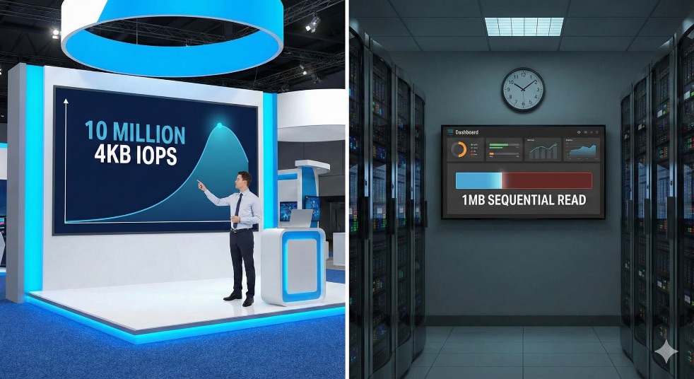
It’s 2012. You’re the person everyone calls when the data is slow. The new flagship OLTP database just went live on a premium all flash array. The vendor flew in engineers, ran demos, and plastered “10 million 4KB IOPS” across every slide. The CIO signed the PO partly because of that number.
Yet tonight, the database is fine. What’s broken is everything around it.
The data warehouse job that populates the CFO’s morning dashboard is still running. ETL that once finished at 4 a.m. now drifts toward midmorning. Analysts stand in the kitchen with coffee, refreshing reports that stubbornly show data as of yesterday.

IOPS aren’t the problem. The problem is that your world doesn’t look anything like the benchmark your storage was sized against.
You know, deep down, that 4KB numbers don’t tell the real story. But at this point, the industry doesn’t have better language. Your storage vendor celebrates their benchmark wins. Your CIO congratulates herself on the procurement decision. Your database team is satisfied. But your data warehouse team, the people who actually drive business value, sits in meetings watching clock hands move while yesterday’s data trickles in.
**The times, as it turns out, are about to change. But first, you have to understand how we got here.**
Chapter 1: Living in the 4KB World (While OLAP Starved)

In those early flash years, the narrative is simple: more IOPS equals more performance. Everything, from RFPs to tradeshow booths revolves around 4KB random reads. It sounds authoritative and technical, and it gives people something to compare.
But here’s the truth nobody talks about: **4KB random IOPS are an OLTP metric.** They measure index probes, log writes, and tiny transactional updates. They tell you almost nothing about OLAP workloads, the analytical queries, warehouse scans, and batch jobs that actually consume most of your storage bandwidth.
When you profile your jobs in detail actually run trace tools and measure what’s happening, you see 128KB and 1MB blocks dominating the landscape. 4KB appears like seasoning, not the main dish.
The OLTP system does exactly what the vendor promised. Index lookups are fast. Tiny, random IO hums along. Database administrators are happy.
Yet when you walk over to the analytics team, the story changes completely:
– **Nightly fact table loads** run on large, sequential blocks 1MB chunks flowing out of staging areas into the warehouse
– **Reporting queries** churn on full table scans where entire indexes get read sequentially
– **Batch jobs** read and write hundreds of gigabytes at a time
– **Month end closing** requires scanning terabytes of transactional data
– **Year end reconciliation** means sequential reads that dwarf any random IO pattern by orders of magnitude
In OLAP terms, a “10M 4KB IOPS” slide tells you almost nothing about scan speed across terabytes, join performance, or how fast you can rebuild a cube or refresh a CFO dashboard.
The array that wins the benchmark bake off doesn’t necessarily win your real workload. In fact, sometimes the opposite happens: the system optimized for tiny random reads shows its weakness precisely when you need sequential throughput.
You file this away as “just how it is.” Storage is a tradeoff—one system for OLTP, another for analytics, and a lot of glue in between. But something in you keeps wondering: **what if storage didn’t have to be this fragmented?**
Chapter 2: The Spark Years and the Tiering Maze

Fast-forward to 2017. Your world has grown considerably. Now there’s a Spark cluster sitting in your infrastructure. Data scientists have appeared, dozens of them bringing Python notebooks and ambitious expectations.
Instead of one big warehouse controlled by a central team, you have a lake full of Parquet and ORC files, growing daily, accessed by teams across the organization. Queries run over terabytes, sometimes petabytes, of data. Machine learning models train on historical data. ETL pipelines have multiplied.
This is where the gap between benchmarks and reality becomes impossible to ignore. **These are all OLAP-style workloads**, large sequential scans, columnar formats, complex aggregations and they depend on sustained throughput, not tiny IOPS.
The analytics team doesn’t care about 4KB anything. They care about:
– How quickly a Spark job can scan billions of rows when executing a complex aggregation
– Whether exploratory queries run in seconds or minutes when they’re iterating on a hypothesis
– Whether they can run five different model training jobs in a day or whether they’re limited to one careful, scheduled attempt
– Why a query that should take five minutes takes forty five when executed against your storage
You sit with them in troubleshooting sessions. They show you job logs. **The CPU cores sit idle while IO completes.** The network interface isn’t saturated. The issue isn’t network congestion. It’s storage throughput, the platform simply cannot feed data to the Spark executors fast enough to keep them busy.
The Tiering Answer

The storage answer you’re given is tiering. “Put hot data on fast tiers. Warm data on NAS. Cold data on object storage. Archive the rest.”
So you adopt it. You build it. You create automation to move data between tiers. You write policies about what lives where.
Soon, your environment looks like this:
– A block array for databases and hot OLTP data
– A NAS fleet for file shares, metadata, and some hot analytics
– An object store for the data lake where Parquet files live
– A separate analytics appliance for warehouse queries
– An archive tier for compliance and historical data
Every new project triggers a conversation: *Where does this data belong?* Every new workload requires a decision about which tier to start with. A typical pipeline looks like: ingest to object → land to file → stage to block for analysis → export back to object for sharing. **Each hop means copies, data validation, new failure modes**.
You’ve gone from one problem: “my storage doesn’t match my workload” to five separate problems glued together with custom orchestration.
And still, performance conversations keep coming back to IOPS and point benchmarks that never quite match your real OLAP jobs.
Chapter 3: When AI Arrives and Breaks Everything

Then AI shows up. And it doesn’t politely integrate into your tiered architecture. **It breaks it.**
At first it’s small and experimental, a few GPUs in a lab box, models that fit comfortably on NVMe inside a single server. Nobody expects it to last.
But curiosity becomes pilot, and pilot becomes platform. Suddenly your board is approving capital for GPU clusters. You’re signing contracts for racks of DGX servers, each costing half a million dollars.
Training jobs stream massive datasets continuously. A trillion parameter language model needs to read the same data multiple times during training epochs. Checkpoints write 14 terabytes every two hours, complete model weights, optimizer states, training metadata.
You sit in a design workshop with your GPU vendor. They talk about feeding GPUs at hundreds of gigabytes per second. They explain that stalls in the data pipeline translate directly to GPU idle time and at $10,000 per GPU per day in cloud terms, idle GPUs become very expensive, very fast.
At that moment, you realize something uncomfortable: **your tiered storage estate was never designed for this workload pattern.**
The architecture assumes cold data, periodic access, acceptable latency in the hundreds of milliseconds. AI training assumes hot data, continuous streaming access, sub-millisecond latency requirements. The gap is fundamental.
The Pilot That Revealed the Truth
The first training run is exhilarating. GPUs light up. Utilization metrics show 85% occupancy. The model trains.
Then, as real usage patterns emerge:
– Checkpoints start to drag.** A 14TB state that should flush in minutes takes an hour or more. GPU clusters sit idle waiting for IO
– A drive failure triggers rebuilds** that cut throughput in half for hours—that one failure cost you $100K in lost compute capacity
– Agent version mismatches** during an OS upgrade cause intermittent node failures. Debugging consumes two weeks of engineering time
– New data pipelines need integration** with three different systems: the AI storage, the traditional analytics tier, and the object lake
Suddenly IO becomes the pacing factor of the most expensive system you’ve ever deployed. You have racks of GPUs that cost millions of dollars **waiting for storage IO**.
You begin to wonder: what if there was a different way?
Chapter 4: When OLAP and AI Exposed the Benchmark Lie

Around this time, you encounter VAST Data. Not through sales email, but through a customer who runs their AI infrastructure on VAST. They mention, casually, that checkpoint writes that used to take 45 minutes now complete in 6 minutes. That GPU utilization improved from 68% to 91%. That they eliminated three separate storage platforms.
You’re skeptical. Every vendor makes claims. You’ve heard promises before.
**But you run a test.** Not a vendor controlled benchmark. A side by side test using your actual patterns, not 4KB random reads, but a mixture of 1MB training data loads, 128KB analytical queries, and 14TB checkpoint writes.
### The OLAP-Relevant Results
| IO Pattern | Local SSD | VAST Cluster | Advantage |
|————|———–|————–|———–|
| 1MB sequential reads | <5 GiB/s | 50+ GiB/s | **10x** |
| 128KB analytical reads | 3-4 GiB/s | 46+ GiB/s | **13x** |
| 1MB sequential writes | 0.9 GiB/s | 11 GiB/s | **12x** |
The tiny 4KB tests still look flattering for SSD. VAST shows competitive but not dominant performance there.
**But when you overlay those results with actual job profiles from your clusters, the story flips completely.** Almost all of your critical throughput lives in the 128KB–1MB space where VAST is multiple times faster. The 4KB pattern that dominated the benchmarks you’ve been reading for fifteen years accounts for maybe 2% of your actual storage IO.
It’s like realizing that your whole career, you’ve been judging cars by how quickly they can parallel park, while what you actually needed was highway speed and fuel (or battery) range.
This benchmark reframes the entire conversation:
– Instead of “how many IOPS?” you start asking **”how many TB/s can I sustain for hours while feeding GPU clusters?”**
– Instead of “how many tiers?” you ask **”why aren’t all my workloads on one system if the performance is better?”**
– Instead of “which agent version is compatible with which OS?” you ask **”why do agents exist here at all?”**
Chapter 5: Discovering a Different Kind of Architecture

When you look under the hood of that VAST system, the differences are structural, not cosmetic. This isn’t a faster version of what you already have. **This is a fundamentally different design**.
The DASE Architecture
**CNodes (Compute/Protocol Layer):** Stateless frontend nodes speak all the languages your applications need—NFS for file access, SMB for Windows shares, S3 for object protocols, NVMe/TCP for direct block access, even GPU-Direct Storage for DMA transfers that bypass CPU entirely. No kernel drivers installed on your hosts. No compatibility matrices.
**DNodes (Capacity Layer):** Backend nodes own pools of dense QLC flash, treated not as blocks and LUNs but as a sea of fine-grained elements. Data isn’t owned by a particular RAID set or controller. Every C-node can reach every piece of data with no fixed affinity.
**NVMe Fabric:** The connection isn’t a traditional SAN protocol limited by distance and latency. It’s NVMe-over-TCP at TB/s speeds per rack, clustered globally, with linear scaling.
Global Similarity Reduction

Data reduction isn’t an afterthought bolted onto the side. It’s baked into the architecture. The similarity engine finds patterns across terabytes of data—repeated model checkpoints, duplicated Parquet partitions, common container layers—at 4K-128K granularity across the entire global namespace.
**Protection** isn’t about carving RAID sets and praying rebuilds finish before business hours. Erasure coding spans wide across nodes—14+2 distribution means any two nodes can fail and the system continues at full speed.
You notice what **isn’t** there:
– No kernel drivers deployed on your GPU nodes
– No compatibility matrix between host OS version and storage plugin version
– No separate AI tier, analytics tier, database tier, and backup tier
– No agents consuming CPU cycles while your models train
– No licensing per protocol
Chapter 6: VAST Database, The OLAP Engine Built Into the Platform

Here’s where the story takes another turn. VAST isn’t just unified storage. **It includes a native database engine designed to eliminate the OLTP/OLAP divide entirely**.
Breaking the OLTP/OLAP Tradeoff
Traditional architectures force you to choose: row-based databases optimized for fast, small transactions (OLTP), or columnar systems designed for large-scale analytical scans (OLAP). You end up with separate systems, ETL pipelines to move data between them, and all the latency and complexity that entails.
VAST Database combines both capabilities into a single system:
– **Transactional properties** for real-time data ingestion—ACID-compliant, with transaction boundaries that can span multiple tables
– **Columnar storage format** optimized for analytical queries—data transforms from standard record form into columnar objects during the write path
– **32KB atomic objects** that enable fine-grained access—when you query the system, it retrieves precisely the data you need, making the system extremely fast for both fine-grained operations and large scans
Native Integration with Analytics Engines
VAST Database supports native SQL querying and integrates with popular query engines through push-down plugins:
– **Apache Spark** push-down for accelerated lakehouse queries
– **Trino** integration for federated analytics
– **Dremio** support for self-service BI
When your Spark job queries data stored in VAST, the query logic pushes down to the storage layer. Instead of pulling raw data across the network and processing it on Spark executors, the heavy lifting happens where the data lives.
The Write Buffer Architecture
VAST Database uses a write buffer in storage-class memory—the fastest persistent media available—to absorb incoming data. This provides time for data manipulation before storing it in low-cost QLC flash.
During this process, data transforms from standard database record form into a columnar format optimized for analytics. The result: you can ingest transactional data at high speed while simultaneously running analytical queries against the same dataset.
Real-Time OLAP Without ETL
The traditional data warehouse pattern looks like this: OLTP database → nightly ETL → staging → warehouse → BI tool. Each step adds latency. By the time analysts see data, it’s hours or days old.
With VAST Database, **the transactional system and the analytical system are the same system**. Data ingested for operational purposes is immediately available for analytical queries. The CFO dashboard that was running on yesterday’s data can now run on data from minutes ago.
Vector Search at Scale
For AI workloads, VAST Database includes vector storage capabilities designed for trillion-scale vector search. Key characteristics:
– Real-time search and retrieval across operational, analytical, and vector workloads
– Constant-time search across large vector spaces
– Native integration with embedding models for RAG applications
This isn’t a separate vector database bolted onto the side. It’s part of the same unified platform that serves your block storage, file shares, and object lake.
Chapter 7: Watching Your Workloads Transform

The first real change you notice isn’t on a benchmark chart. It’s in how your workday feels.
Spark and Analytical Workloads
Your Spark jobs that once required careful staging to local SSD—staging that consumed both engineering time and storage space—start running directly against the VAST cluster. The 128KB and 1MB scans that used to saturate servers and cause cluster-wide pauses now complete in a fraction of the time.
Rerunning a full pipeline goes from “schedule it overnight and check results in the morning” to “kick it off at 10am and have results by lunch.” **Iteration becomes practical.** Data scientists can explore hypotheses instead of waiting for batch windows.
AI Training and Inference
Your AI training runs stop treating IO as a rare resource. You stream datasets at speeds that keep GPUs busy instead of hungry. The pattern appears immediately: **GPU utilization climbs from 68% to 92%**.
That’s not a rounding difference. That’s GPU clusters that are actually busy, actually training, actually productive. Your $10M annual GPU investment starts returning value proportional to the investment.
Checkpoints no longer dictate the rhythm of experimentation—they happen in the background during training instead of defining the training pace.
Database Consolidation
Your databases stop being privileged snowflakes that need their own pet storage arrays. You provision NVMe/TCP volumes from the same pool that powers everything else. The same storage that feeds your Spark clusters, stores your AI checkpoints, and serves as your object lake now handles your database IO.
With VAST Database, you can go further: eliminate the separate OLTP and OLAP systems entirely. Ingest transactional data and query it analytically from the same platform, with columnar storage and push-down acceleration built in.
The Object Lake Unification
The object lake that used to live in separate hardware now shares the same platform. S3 reads hit the same NVMe flash as native block. Your Parquet files stored as objects perform identically to files accessed through NFS.
**You quietly retire migration scripts** because you no longer need to bounce data between tiers to make it usable.
Chapter 8: The Human Impact

The technical story is compelling, but the human impact is what sticks with you.
**The storage team** that once spent nights babysitting rebuilds and tracking agent versions finds itself with time for strategy instead of firefighting. They become partners in planning infrastructure, not obstacles to work around.
**Data scientists** notice the shift immediately. Their experience transforms from “open a ticket, wait for infrastructure team, point at a NAS mount, run your query, wait for results that never come” to “point at this bucket/share/volume and go.” The friction between idea and experiment shrinks from weeks to days.
**Your finance team** starts noticing different numbers. The GPU clusters that used to have 60% utilization now run 90%. That’s 50% more effective use of hardware. A 256-GPU cluster effectively behaves like a 384-GPU cluster.
You also see something more subtle: **trust returning to storage conversations.** For years, performance numbers felt negotiable fast in one corner case, slow everywhere else. Now, when you say “this platform can feed 256 GPUs” or “this system will compress your lakehouse by 12x,” you have production behavior to back it up.
Chapter 9: What OLAP Workloads Actually Need in 2026

Standing in 2026, with all these lessons behind you, the requirements for analytical workloads have crystallized:
Throughput Over IOPS
Modern OLAP workloads—Spark SQL, Trino queries, warehouse scans, ML feature engineering—are characterized by large sequential scans, 128KB–1MB IO sizes, and multi-TB datasets. The metric that matters is **sustained throughput**: 140+ GB/s per rack, multiple racks clustered together delivering TB/s. Not peak throughput in ideal conditions—sustained, predictable, available-every-day throughput.
Unified Data Access
A single platform should serve all protocols from the same storage. There’s no “which tier should this data live on?” question because it’s all the same tier. OLAP queries against Parquet in S3, OLTP transactions against NVMe/TCP volumes, and ML training against NFS shares—all from the same capacity pool.
Native Query Acceleration
For analytical workloads, the database engine matters as much as the storage layer. VAST Database provides columnar storage, push-down query execution, and native integration with Spark and Trino—eliminating the ETL tax that traditional architectures impose.
Inline Data Reduction
OLAP workloads often involve repetitive data: similar schemas, duplicated Parquet partitions, versioned datasets. Global similarity reduction captures this automatically, achieving 5-15x reduction factors without sacrificing performance.
Zero Agent Architecture
Every protocol works natively. No custom drivers. No compatibility concerns between OS versions. No agent upgrades that require coordination with security patches.
Epilogue: Looking Back at the Red Dashboard

If you could visit that 2012 version of yourself, the one staring at the stuck ETL job and the triumphant IOPS slides, you’d have a lot to say.
You’d tell them that the real story was never about a single metric, a single protocol, or a single array. It was about all the workloads that would one day converge and demand service simultaneously: OLTP databases with random access patterns, **analytical warehouses with sequential scans**, data lakes with mixed access patterns, AI training with streaming requirements, inference with latency constraints.
You’d explain that architecture, not clever caching, not another tier, not agent density, is what ultimately changes the game. That once you have a platform capable of feeding GPUs at TB/s, serving warehouses with **13x performance advantage** on OLAP style scans, and maintaining databases with native protocols, all from the same pool, questions about “which system owns which workload” simply disappear.
You’d tell them about VAST Database: how the OLTP/OLAP divide that seemed fundamental turned out to be an artifact of architectural limitations, not a law of physics. How columnar storage and transactional capabilities can coexist. How push-down query engines eliminate the ETL pipelines that once consumed entire teams.
Most of all, you’d reassure them that the frustration they felt—the sense that the industry was optimizing for the wrong things, that benchmarks didn’t match reality, that storage innovation had plateaued into complexity instead of simplification, was justified.
**The times really were changing. It just took a while for storage to catch up.**
In 2026, block workloads no longer live in a 4KB world. They live in a world of TB/s, shared data, unified platforms, and intelligent reduction. The silly 4KB benchmarks that dominated a decade of vendor marketing have finally been demoted to what they always were: a minor supporting detail for a narrow slice of workloads.
**The red dashboard from 2012 would never be red again.**